Chapter 2 Materials and Methods

2.1 Materials

2.1.1 Chemicals

Table 2.1: Chemicals

Chemical	Company	cat.-no.
Agarose	Roth	6351.2
Agar-Agar	Roth	5210.3
Ampicillin	Roth	K029.2
ATP	Epicentre	E311K
Blocking Reagent	Roche	11096176001
BCIP	Fermentas	R0822
CaCl	Roth	886.1
Calyculin	Sigma	208851
DAPI	Sigma	D9542
DIG RNA Mix	Roche	11277073910
DMSO	Roth	4720.2
EtBr	Roth	2218.3
EtOH	Roth	9065.3
Formaldehyde	Roth	7398.1
Formamide	Roth	P040.1
Glycerol	Roth	3783.2
IPTG	Thermo	R1171
KCl	Roth	P017.1
Low melting point Agarose	Roth	A9539
Maleic Acid	Roth	3810.3
MgSO	Roth	T888.2
MeOH	Roth	CP43.3
MgCl	Roth	2189.1
NaCl	Roth	9265.2
NaHCO	Roth	855.1
NaOH	Roth	6771.3
NGS	Sigma	C6767
p-Formaldehyd	Sigma	P6148
Phenol Red	Sigma	P0290
Propan-2-ol	VWR	20842330
Proteinase K	Roth	7528.4
PTU	Sigma	P7629
Rockout	Sigma	555553
SSC	Roth	1232.1
SU5402	CALBIOCHEM	572630
Torula RNA	Sigma	R6625
Tricaine	Sigma	A5040
Tris Base	Roth	4855.2
Triton-X100	Roth	3051.2
Trizol	Ambion	15596018
Tween20	Sigma	P1379

2.1.2 Solutions

Table 2.2: Solutions

Solution	Company	cat.-no.
Cut Smart Buffer	NEB	B7204S
Generuler 100 bp	Thermo	SM0241
Generuler 1kb	Thermo	SM0311

2.1.3 Antibodies

Table 2.3: Antibodies

Antibody	Company / Provider	concentration	cat.-no.
Anti-Digoxigenin	Roche	1:200	11093274910
Anti-GFP	Torrey Pines	1:200	-
Anti-TAZ (rabbit)	Cell Signaling Technology	1:200	D24E4
Anti-ZO1	Zymed	1:200	33-9100
Alexa Fluor488	Invitrogen	1:500	710369
Alexa Fluor555	Invitrogen	1:500	Z25005

2.1.4 Enzymes

Table 2.4: Enzymes

Enzyme	Company	cat.-no.
BtsCI	NEB	R0647
DdeI	NEB	R0175
HaeIII	NEB	R0108
MnlII	NEB	R0163
NlaIII	NEB	R0125
NsiI-HF	NEB	R3127
Phusion Polymerase	NEB	M0530L
Pronase	Sigma	P5147
Ribolock	Thermo	EO0381
RNase A	Quiagen	1006657
RNase H	NEB	M0297L
SP6 RNA Polymerase	Thermo	EP0131
T4 Ligase	NEB	M0202T
T7 RNA Polymerase	Thermo	EP0111
Taq DNA Polymerase	Invitrogen	10342-020
Taq DNA Polymerase	VWR	733-1301

2.1.5 Molecular Biology Kits

Table 2.5: Molecular Biology Kits

Kit	Company	cat.-no.
EdU Click-iT	Invitrogen	MP 10083
mMessage mMachine Sp6 Polymerase	Invitrogen	AM1340
PCR & Gel Clean-Up	Sigma	NA1020
pGEM-T TA Cloning	Promega	A3600
Superscript III cDNA Synthesis	Thermo	18080051
Wizard SV Gel and PCR Clean-Up	Promega	A9282

2.1.6 Buffers

Table 2.6: Buffers

Buffer
Blocking Reagent (BR)	2% BR in maleic buffer + 5% serum
E3	(52)
Hybridization buffer	50% Formamide + 25 % 20x SSC + 50mg/mL Heparine + mQ
Maleic buffer	250 mM maleic acid + 5M NaCl + 10% 0.1% Tween-20 + mQ
NTMT	5 M NaCl + 1 M MgCl + 1 M Tris pH 9.5 + 10% Tween
PBS	2.7 mM KCl + 12 mM HPO
PBST	PBS + 0.1% Tween20
PBDT	PBS + 1% BSA + 1% DMSO + 0.3% Triton
PFA	4% paraformaldehyde in PBS
P1	50 mM Tris-HCl pH 8.0 + 10 mM EDTA pH 8.0 + 100 µg/mL RNAse
P2	1M NaOH + 10 % (w/v) SDS
P3	3M KOAc pH 5.5
TNT	50 mM Tris-HCl pH 8.0 + 100 mM NaCl + 0.1% Tween-20

2.1.7 Zebrafish lines

Table 2.7: Zebrafish lines

Allele	name	zfin
zf106Tg	cldnb:lyn-gfp	Tg(-8.0cldnb:LY-EGFP)
fu13Tg	cxcr4b(BAC):H2BRFP	TgBAC(cxcr4b:Hsa.HIST1H2BJ-RFP)
nns8Tg	atoh1a:Tom	Tg(atoh1a:dTomato)nns8
fu50	shroom3	-
m1274Tg	hsp70:shr3v1FL-taqRFP	Tg1(hsp70l:shroom3-TagRFP)

2.1.8 ISH probes

Table 2.8: ISH probes

Probe	Sequence
atoh1a	see (38)
deltaD	see (53)

2.1.9 Morpholinos

Table 2.9: Morpholinos

Probe	Sequence	Concentration
MoAtoh1a	see (38, 54)	0.4 ng/mM
p53	see (55)	2 ng/mM

2.1.10 Hardware

2.1.10.1 Mounting Stamp

An stl file for 3D printing can be found at github.com/KleinhansDa/3DModels

Table 2.10: Materials for production of a standardized mounting stamp

Component	Company	cat.-no.
\(\mu\) dish	Ibidi	81,218–200
Stamp	-	-
Preparation needles	VWR	USBE5470
Pasteur Pipettes	Roth	4518
Rubber / Silicone bulb	VWR	612-2327
Microtubes 2 mL	Sarstedt	2691
Heating block	PeqLab	HX2
Microwave oven	Severin	MW7849
Stereo microscope	Leica	M165FC
Transmitted Light Base	Leica	MDG36
Countersunk screw DIN7991, 8 × 20 mm	Dresselhaus (Hornbach)	7662389
Superglue	UHU	509141

2.1.10.2 Spinning Disc Microscopy

Table 2.11: Spinning Disc system components

Component	Company	Product	Specs
Microscope	Nikon	Eclipse Ti-E	fully motorized
PFS	Nikon	Perfect focus system	Z repositioning
XY-table	Merzhaeuser	XY motorized table	1 \(\mu\)m accuracy
Piezo		Piezo Z-table	300 \(\mu\)m scan range
SD system	Yokogawa	CSU-W1	50 \(\mu\)m pattern
Laser		Laser Combiner	see table 2.12
FRAPPA	Revolution	FRAPPA	-
Borealis	Borealis	Borealis	flat field correction
sCMOS	Andor	ZYLA PLUS	4.2Mpix; 82%QE
Immersion	Merzhaeuser	Liquid Dispenser	-

Table 2.12: Available lasers

Lasers	Type	Power
405 nm	diode	100 mW
445 nm	diode	80 mW
488 nm	DPSS	100 mW
561 nm	DPSS	100 mW
640 nm	diode	100 mW

Table 2.13: Available objectives

Objective	Company	Type	Immersion	N.A.	working distance
10x	Nikon	CFI APO	air	0.45	4.00 mm
20X	Nikon	CFI APO	water	0.95	0.95 mm
40X	Nikon	CFI APO	water	1.15	0.60 mm
60X	Nikon	CFI APO	water	1.20	0.30 mm

2.1.10.3 Workstation

Statistical computation and image analysis were done on a Fujitsu Siemens (FS) Workstation CELSIUSM740 with the following hardware components…

Table 2.14: Workstation hardware components

Component	Company	Product	Specs
CPU	Intel	Xeon E5-1660v4	3.2 GHz, 20MB, 8cores
RAM	Fujitsu	-	4x16GB DDR4-2400
Graphics	NVIDIA	Quadro M4000	8GB RAM

2.1.11 Software

Table 2.15: Used software

Software	Version	web
Imagej FIJI	1.48	https://fiji.sc/
R	3.6.1	https://cran.r-project.org/
RStudio	1.0.153	https://www.rstudio.com/
Ubuntu	17.1	https://www.ubuntu.com/
Windows 10 Pro	10.0.16299
Total Commander	9.0	http://ghisler.com/

2.2 Methods

2.2.1 Data Strategy and Analysis

Due to the history of Developmental Biology and the complexity of biological processes per se, the field heavily relies on image data. Since the advent of electronic imaging techniques¹¹ scientific image data can be processed and analyzed in silico. To take advantage of

1. live imaging, which (as compared to fixation techniques) conserves the cellular integrity and morphology while also offers the possibility of recording time-lapses
2. the optically clear specimen and
3. high throughput image analysis and state-of-the-art data science using algorithmic implementations,

the three following points were paid special attention to.

2.2.1.1 Sample Preparation

For fluorescence microscopy zebrafish embryos are usually immersed in a 1\(\%\) solution of low melting-point agarose (LMPA) and then oriented on an optical cover slip manually until the LMPA has solidified. This process allows to mount¹² eight to ten embryos per dish. To make use of the high number of offspring, a single zebrafish female may lay, which rapidly leads to a sample number of more than 300, a new sample preparation technique was designed that allows for (1) a four to five - time increase in samples per dish (2) a facilitated navigation via a grid-like orientation through the samples and (3) an improved spatial orientation where the embryos body axes are aligned parallel to the optical Z-sections of the confocal microscope. For details, see Materials and Methods section 2.2.3.4 and Kleinhans et al., 2019 (56).

2.2.1.2 Imaging

Technically, speed and sensitivity are most important for live imaging. Considering these two parameters a light-sheet (57) fluorescence microscope (LSFM) would be the best fit. However, LSFMs also have several limitations. First, due to the sample preparation methods available, the number of samples that can be imaged at a time is highly restricted. Second, for subcellular resolution a high magnification is required, which is limited by working distances and third - for optimal image analysis a high signal-to-noise ratio (SNR) and numerical aperture (N.A.) is preferable. Therefore a spinning disc (58) system was chosen for most of the imaging. The system makes use of (1) an extra-large field of view (FOV) ideal for large specimen, (2) the possibility of a high degree of automation with state-of-the-art software and (3) a water dispensing system for long-term water immersion imaging. For details about the system see Materials section 2.1.10.2.

2.2.1.3 Data handling

After data acquisition and pre-processing, the image data was transferred from the microscope system to the labs main workstation. To uniquely identify each file and have them appear in a structured manner, a file-naming system was established after the following structure

Where stage would e.g. be 32hpf, group would be a genotype or drug treatment, id would be a positional identifier on an imaging dish like B1P01¹³ and date would be a date in the form of YYMMDD.

2.2.1.4 Image and Data Analysis

In order to be as objective and as high throughput as possible, almost all of the analyses performed for this study was solved either algorithmically or using convolutional neural networks (CNNs). Furthermore, to meet the terms and conditions of open science¹⁴ standards, all pipelines were implemented in open source software frameworks such as Fiji is just image J (FIJI) and R. For further information about training datasets, algorithms and versions used see Materials section 2.1.11.

2.2.2 Zebrafish

2.2.2.1 Husbandry

Zebrafish husbandry was maintained at the University of Frankfurt am Main. All legal procedures were followed while handling and maintaining zebrafish husbandry. All zebrafish lines used in and generated for this study are listed in Materials section 2.1.7.

2.2.2.2 Handling and rearing

In the afternoon preceding the embryo collection, 1 male and female were set up in crossing cages, physically separated by a transparent separator. Next day, before noon, separators were removed allowing fertilization. Fertilized eggs were then collected, sorted and reared in the well-defined culture medium E3 (Kimmel et.al. 1995, section 2.1.6) at 25\(^\circ\), 28.5\(^\circ\), or 30\(^\circ\)C depending on the experimental condition required.

To grow larvae to the adulthood, they were transferred to the system on day 5. Till day 12, larvae were fed Vinegar Eels, Paramecia, and caviar powder. After the 12 th day, water supply was started and fish were fed Brine Shrimp, Artemia, Paramecia and Vinegar Eels. Adult fish (>1 Month) were fed Artemia and the dry flakes.

2.2.2.3 Zebrafish fin clips

Adult fish were anesthetized with buffered Tricaine (1X, see section 2.1.6) until loss of motion. About 1/3 of the caudal fin was cut with a sterile scalpel in a sterile Petri Dish. Immediately the dissected fin was transferred to 100 \(\mu\)L of 50 mM NaOH. Fish were returned to system water and kept in 1L system water in single tanks with 200 \(\mu\)L of 0.01\(\%\) Methylene Blue.

2.2.2.4 Adult Genotyping

The clipped fins were digested for 1 h at 95\(^\circ\) C and neutralized subsequently with 10 \(\mu\)L of 1M Tris-HCl of (pH 9).

2.2.2.5 Embryo Genotyping

Single fixed/live embryos were denatured at 95\(^\circ\) C in 20 \(\mu\)L of 50 mM NaOH for 1 hour and neutralized by adding 2.5 \(\mu\)L of 1 M Tris-HCl (pH 9).

2.2.2.6 Zebrafish Euthanasia

Adult zebrafish were euthanised by an overdose of Tricaine in ice cold water so as to sacrifice them by hypothermia.

2.2.2.7 Fixation

Embryos and dechorionated larvae were fixed in 2 mL of 4\(\%\) PFA in 1X PBS overnight at 4\(^\circ\) C.

2.2.3 Wet lab

2.2.3.1 Sample preparation

For samples older than 24 hpf, embryos were grown in 1X PTU till desired stage and treated with 150 \(\mu\)L per 10 mL of 0.1 mg/mL Pronase for ~30 min.. Choria were removed by gentle pipetting with a 2 mL plastic pasteur pipette. To replace the Pronase solution with fresh E3, embryos were immobilized by anesthesia and collected in the center of the dish by gentle rotational movement. Then the medium was decanted by collecting the embryos at the corner bottom of the dish while taking care not to loose any. After, the dish was filled with fresh E3. This process was repeated three times.

For samples younger than 18s stage, embryos were treated with 150 \(\mu\)L per 10 mL of 0.1 mg/mL Pronase directly. Choria were removed the same way as for > 24 hpf embryos but when pouring away the Pronase solution, the dish was simultaneously and very carefully filled with fresh E3 again. Since younger embryos are more fragile and to avoid damage, they must be kept in solution constantly.

Fixation started at the desired stage in 4\(\%\) PFA in 0.1\(\%\) PBST in 2 mL tubes at 4\(^\circ\)C o.n.. The next day, samples were rinsed 3 times for ~5 min. in PBST and passed through a MeOH series of 25\(\%\) \(\rightarrow\) 50\(\%\) \(\rightarrow\) 75\(\%\) \(\rightarrow\) 100\(\%\) MeOH/PBST (V/V)). For permanent storage, samples were stored in 100\(\%\) MeOH at -20\(^\circ\)C.

2.2.3.2 In Situ Hybridization

Samples were prepared after the method described in section 2.2.3.1.

2.2.3.2.1 1. Permeabilisation & Probe Hybridization

Permeabilisation \(\rightarrow\) without shaking

Samples were rehydrated in an inverse MeOH series of 75\(\%\) \(\rightarrow\) 50\(\%\) \(\rightarrow\) 25\(\%\) \(\rightarrow\) 0\(\%\) PBST and washed again for fice min. two times in pure PBST. Finally, samples were digested in 10 \(\mu\)g/mL Proteinase K according to table 2.16.

Table 2.16: Proteinase K digestion

Stage	0.6 s	7 s	18 s	24 hpf	32 hpf	36 hpf	42 hpf	48 hpf	72 hpf
min.	0	4	6	15	30	40	50	60	60

Samples were rinsed again two times in PBST and post-fixated in 4\(\%\) PFA at 4\(^\circ\)C for > 30 min. Samples were washed again for 5 min. three times in PBST.

Probe Hybridisation \(\rightarrow\) all steps at 60\(^\circ\)C, except stated differently

Samples were pre-hybridized in 350 \(\mu\)L of hybridization buffer (section 2.1.6) for 1 - 8 h. Just before detection probe treatment, the probe was denatured at 80\(^\circ\)C in 1:200 of hybridization buffer. Subsequently, hybridization buffer was taken off the samples and replaced with the heated probe. Finally, samples were incubated o.n. at a desired temperature (around 65\(^\circ\)C).

2.2.3.2.2 2. Probe removal & Antibody incubation

The next day the probe got collected and stored at -20\(^\circ\)C for re-use. Washing took place at the same temperature as hybridization (from step 1) To keep solutions at temperature a Thermo-Block was used. For the washing series the samples were first washed one time for 20 min. in hybridization buffer, then two times for 30 min. in 50\(\%\) Formamide and one time for 20 min. in 25\(\%\) Formamide. Then two times for 15 min. in 2X SSCT and two times for 30 min. in 0.2X SSCT. Finally, one time for 5 min. in TNT.

To reduce noise and increase specific signal strength, the samples were treated with blocking solution (section 2.1.6) for 1 - 8 h in 350 \(\mu\)L of 2% BR/TNT at room temperature (RT). Afterwards the samples were incubated in 100 \(\mu\)L Anti-Digoxigenin diluted in NTMT buffer (1/4000 (V/V)) in 2\(\%\) BR/TNT for 2 h at RT or o.n. at 4\(^\circ\)C.

2.2.3.2.3 3. Probe detection

First, the samples were washed six times for ~20 min. (or one wash o.n.) in TNT and two times for ~ 5min. in NTMT. After washing, color staining was performed with 4.5 NBT \(\mu\)L + 3.5 \(\mu\)L BCIP per mL NTMT in the dark and at RT without shaking (in a drawer) for 2 - 8 h, regularly checking the progression of the reaction. As soon as an appropriate degree of color intensity on the target site was achieved (up to two days), the samples were again washed three times in PBST.

Afterwards the samples were either prepared for immunostaining or imaging. For permanent storage samples were kept in 50\(\%\) Glycerol at 4\(^\circ\)C.

2.2.3.3 Immuno staining

Samples were prepared after the method described in section 2.2.3.1.

First, samples were blocked in 2\(\%\) Goat Serum / PBDT (V/V) for 30 min.. For protein target site detection, a primary antibody (150 \(\mu\)L of 2% NGS / PBDT (V/V)) was incubated for ~2 h at RT or o.n. at 4\(^\circ\)C. Samples were washed for 2 h in PBDT while changing the solution 5 - 6 times. To stain the now bound primary antibody, a secondary antibody (150 \(\mu\)L of 2% NGS / PBDT (V/V)) was incubated for 2 h at RT or o.n. at 4\(^\circ\)C. Samples were washed for 2 h in PBDT while changing the solution 5 - 6 times.

2.2.3.4 Mounting

For live microscopy zebrafish embryos are usually immersed in a 1\(\%\) solution of low melting-point Agarose (LMPA) solution and then oriented on an optical cover slip manually until the LMPA has solidified. This process allows to mount eight to ten embryos per dish.

To take advantage of the high number of offspring a single zebrafish female may lay, a new sample preparation technique was designed that allows for

1. a four to five times increase in samples per dish
2. a facilitated navigation via a grid-like orientation through the samples and
3. an improved spatial orientation where the embryos body axes are aligned parallel to the optical Z-sections of the confocal microscope.

A detailed protocol can be found under section 3.1.1

2.2.4 Dry lab

2.2.4.1 Image J macros

Three IJ macros have been developed to facilitate image analysis and make results more reproducible. Each of them is specifically designed for input of LL and pLLP images of the cldnb:lyn-gfp transgenic line.

Hence, they are called anaLLzr …

• 2D - analysis of Z-projected images of the LL at end of migration
• 2DT - analysis of Z-projected images of the LL during migration
• 3D - analysis of 3D image stacks of the pLLP at a given timepoint

Since their development was an integral part of my PhD work, the description of the macros can be found in the results part in section section 3.1.

2.2.4.2 Proliferation Analysis

The basic principle is based on work done by Laguerre et al., 2009 (34). For registration of mitotic events an IJ manual tracking tool was used that allows to track an image feature through a stack of images creating tracks as it progresses through volume / time (‘MTrackJ’(59)).

For mounting the embryo, the procedure described in section 2.2.3.4 was used. Nuclei were visualized in a TgBAC(cxcr4b:H2B-RFP) transgenic line. After Z-projection of volumetric timelapses, mitotic events were tracked in each CC and the pLLP. Afterwards the data was exported as one table per embryo and processed by counting mitoses per pLLP / CC / total CC mitoses. Figure 2.1 shows an exemplary track for the data analyzed.

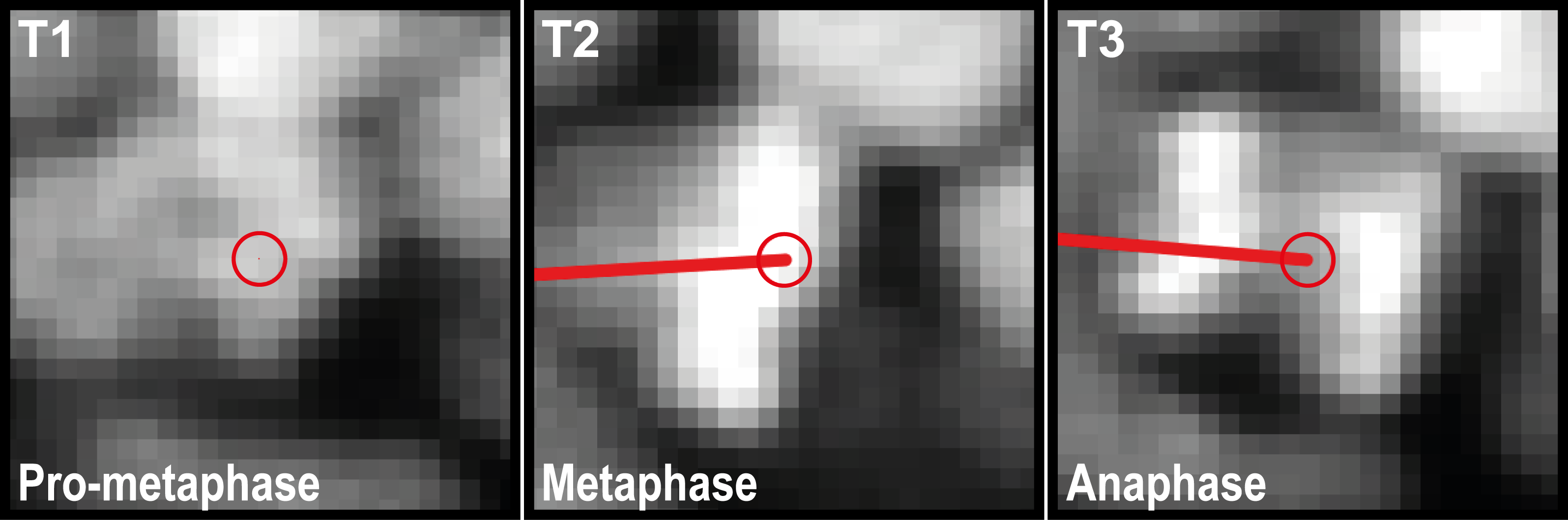
Figure 2.1: Tracking of mitotic events. T1-T3 show consequetive timepoints of a single nucleus.

2.2.4.3 Apical Index

2.2.4.3.1 Rationale

The earliest attempt found for indexing AC can be found in a study published by Lee et al(60) where they were interested in the ‘apical index’ (A.I.) of bottle cells during X.laevis gastrulation (figure 2.2 Lee). Another example for measuring AC is the apical constriction index (A.C.I., figure 2.2 Harding) for the cells of the D.rerio lateral line primordium (pLLP), which can be found in a study from 2012 where it was shown that FGFr-Ras-MAPK signaling is required for Rock2a localization and AC (61, 62).

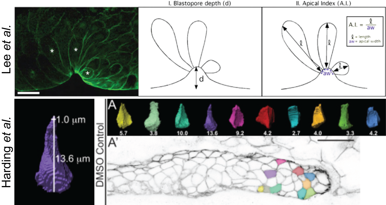
Figure 2.2: A.I. indeces in the literature. Lee A.I. of X.leavis bottle cells measured in 2D. Harding A.I. of D. rerio pLLP cells measured in 3D.

In these two publications, the way they measure A.I. (60) and ACI (62) respectively, does not differ and is the ratio of lateral height over apical width.

\[\mathbf{ACI} = \frac{lateral\;height\;[\mu m]}{apical\;width\;[\mu m]}\]

We found two principal weaknesses of applying this ratio to the cells of the pLLP. First, it does not respect the independence of lateral height to AC. Second, it does not differentiate between constriction along the anterio-posterior (AP) or the dorso-ventral (DV) axis. Third, it actually represents the A.I. rather than the apical constriction index.

2.2.4.3.1.1 Parameter definition

To obtain a precise and biologically meaningful way to quantify AC, first a couple of definitions had to be made.

Definition 2.1 (AC is independent of orientation) In a 3D space a cell can have any orientation and still be apically constricted. Therefore, before measuring one should make sure orientation between embryos is aligned and also consider taking measurements along two different directions. Since apical constriction is not necessarily isotropic, it is important to consider constriction along 2 perpendicular axes (AP and DV axis of the embryo/pLLP).

Definition 2.2 (AC is independent of lateral height) Lateral height can be described as the distance of the two farthest points on the surface area of a cell. Two cells with different lateral heights can be equally apically constricted.

Definition 2.3 (AC is independent of cell volume) The volume of a cell represents its size. A large cell can be equally constricted as a small cell.

2.2.4.3.1.2 Adaption for variation in lateral height

To test different A.I. conditions, an apically constricted cell can be approximated by modeling a tetrahedron. For example, shrinking or enlarging a cell symmetrically should not affect the A.I.. As described by Harding(2014)(62), the apical width of a cell is measured first by manual 3-D reconstruction, second manual re-orientation, and third by going 1 \(\mu\)m from the apical tip into the cell (from now on referred to as \(\Delta\)ap, 2.3B). Finally, apical width is the total width of the 2D object in the respective volume.

If \(\Delta\)ap is a constant, the A.I. in a symmetrically enlarged cell increases from e.g. ~15 to ~23, since apical width stays the same but lateral height increases (compare figure 2.3A to A’). On the contrary, if \(\Delta\)ap is adjusted relative to a cells lateral height, e.g. by percentage, the A.I. in a symmetrically enlarged cell stays the same (compare figure 2.3A to A’’).

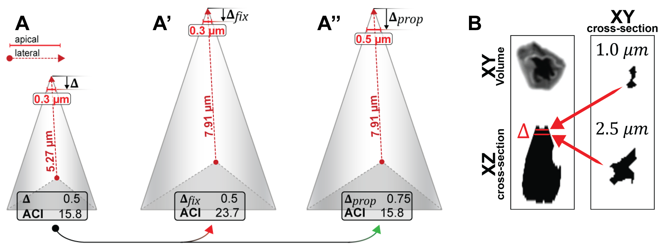
Figure 2.3: Different ways to quantify the apical index. A-A’’ A.I. Cell Models. A’ and A’’ show cells that are symmetrically increased versions of A. While in A’, constant delta was used, in A’’ delta is proportional to the lateral height. B Illustrating delta ap. (left) apically constricted cells volume rendered in XY (top) and as a lateral cross-section in X-Z (bottom). (right) 2-D area as seen at \(\Delta\)ap of 1 or 2.5 \(\mu\)m.

Therefore the measurement for apical width has to be relative to lateral height.

\[\mathbf{ACI} = \frac{lateral\;height\;[\mu m]}{relative\;apical\;width\;[\mu m]}\]

2.2.4.3.1.3 Adaption for tissue polarization

Organs develop in a 3-D space and are polarized along each axis. AC usually describes a 2-D morphogenetic movement towards a center along the X-Y axes. However, the constriction movements along X and Y might be independent of one another. This could mean that they happen at different speeds, or that one is absent. As a result, the tissue would look less radially (figure 2.4B) constricted, but more constricted along one particular axis (anisotropic). In order to separate those two AC dimensions, the A.I. can be calculated for the anterio-posterior and for the dorso-ventral axis (figure 2.4, horizontal vs. vertical).

Figure 2.4: Schematic AC along the A-P and D-V axis. A shows a A-P and D-V constricted cluster of cells. B shows a D-V constricted cluster of cells.

By fitting an ellipsoid to the area taken at \(\mathrm{\Delta}\)ap, one will obtain the following parameters (figure 2.5).

1. Length of Major axis
   • indicates the level of constriction along the less constricted axis
2. Length of Minor axis
   • indicates the level of constriction along the most constricted axis
3. Angle of Major from 0\(^\circ\)
   • indicates the orientation of the long, less-constricted axis: If the angle is close to 0\(^\circ\), the long axis of the apical area is parallel to the AP axis (the cell is constricted along the DV axis). If the angle is close to 90\(^\circ\), the long axis of the apical area is parallel to the DV axis (the cell is constricted along the AP axis).

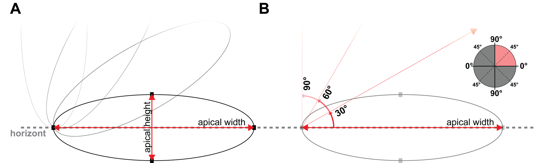
Figure 2.5: Scheme of ellipsoid measures. A shows the major axis as apical width and the minor axis as apical height. B shows the angular displacement from the horizon in steps of 30\(^\circ\).

2.2.4.3.1.4 Measurement definition

The two dimensions of A.I. indices can therefore be defined as the following ratios…

Definition 2.4 (A.I. Major) \[\mathbf{A.I._{Major}} = \frac{lateral\;height\;[\mu m]}{ellipsoid\;major\;axis\;at\;relative\;\Delta ap\;[\mu m]}\]

Definition 2.5 (A.I. Minor) \[\mathbf{A.I._{Minor}} = \frac{lateral\;height\;[\mu m]}{ellipsoid\;minor\;axis\;at\;relative\;\Delta ap\;[\mu m]}\]

Definition 2.6 (Angle Major) \[\mathbf{Angle_{Major}} = \measuredangle = \mathrm{\Delta}\;from\;horizon\;[0-90^\circ]\]

2.2.4.3.2 Measurements

As a proof of principle of the definitions stated in the previous section we compare our results to previously published results from Harding et al. (61) who, as a control, measured apical constriction in embryos treated with an FGF inhibitor (SU5402) and their DMSO controls.

2.2.4.3.2.1 Single cell measurements

Each geometric object has a centroid coordinate in X and Y (and Z) which is represented as the mean of all X or Y coordinates within the object. In figure 2.3, centroid coordinates in X and Y are used to plot the cells as points in the X-Y plane. Additionally, each point is colored for the A.I. value (high values are dark red - red, middle values are green, low values are cyan - blue).

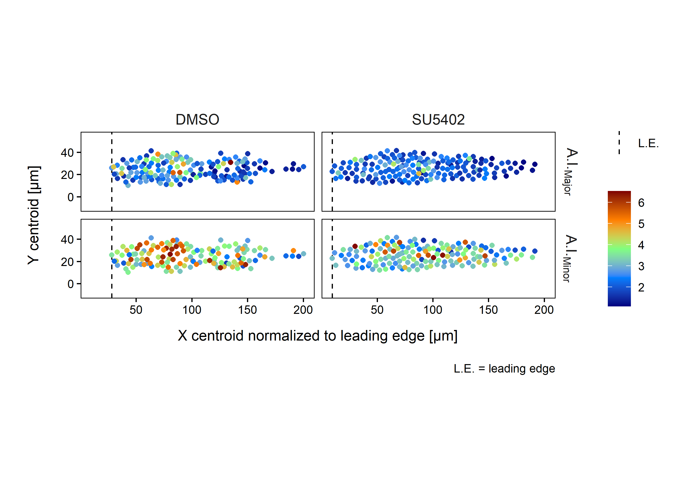
Figure 2.6: A.I. single cell measurements

Harding et al. (62) were using a constant \(\mathrm{\Delta}\)ap to measure the apical width, which we have shown to be incorrect in certain cases. In their study they found that certain mean A.C.I. values in the DMSO go as high as 15 (figure 2.7), which might be related to this (see figure 2.3). By measuring apical width at a relative \(\mathrm{\Delta}\)ap and taking into account all pLLP cells of the two exemplary pLLPs shown in figure 2.3, we measure a mean difference in the Major of 0.53 and 1.11 in the Minor.

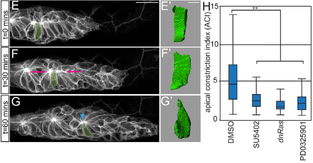
Figure 2.7: A.I. indices by Harding et al. E-G’ 3-D reconstructions of the highlighted cell. H A.C.I.s for embryos treated with DMSO, SU5402, PD0325901 or following induction of hsp70:dn-Ras. (n = 180 cells / N = 6 embryos).

2.2.4.3.2.2 Angle densities

To check whether there is a bias in orientation of the apical width, the angle measurements 2.5 can be shown as a function of density along X (figure 2.8A).

Interestingly the results indicate that there is less of a difference for the Major_Angle at angles bigger than 15-20\(^\circ\). This would mean that the apical surface of the cells in SU5402 treated embryos is more strongly oriented along the horizontal antero-posterior axis.

2.2.4.3.2.3 ACI magnitude at different angles

Now, to get an idea of the magnitude of constriction relative to the orientation of the cell (angle to the horizontal), the A.I._Major/Minor can be shown as a function of the Major_Angle (figure 2.8B-B’).

Since AC is a 3-D morphogenetic process and since cells in a wild type pLLP are mostly radially organized, it does make sense to look at AC from more than just one perspective. Here we propose to separate the A.I. into an antero-posterior and a dorso-ventral dimension.

1. While for the control (DMSO treated) embryo the distribution of the cells Major Angles seem to be mostly uniform, for the SU5402 treated embryo there is an accumulation of lower Major Angles. This means that cells in SU5402 treated embryos are more oriented along the horizontal (anterior - posterior) axis.

2. Interestingly there does not seem to be much of a difference in A.I._Major (figure 2.8B), which can also be shown by the mean values which are at 2.6 for the DMSO control and at 2.1 for the SU5402 treated condition.

3. For the A.I._Minor (figure 2.8B’) the means are 4.7 for the DMSO control and 3.6 for SU5402. The base constriction for both, DMSO and SU5402 is at around 3.6, however there is a peak at around 40 - 60\(^\circ\) in the DMSO control where cells are most constricted having a maximum A.I. at 15.8. This indicates that for the Minor, cells in that range of angles are more constricted than cells oriented in different directions.

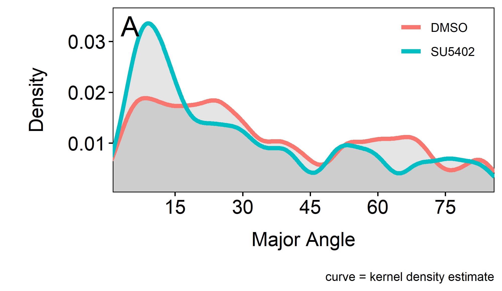
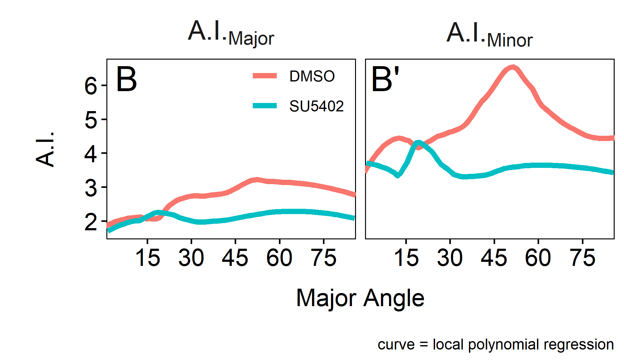
Figure 2.8: A.I._Major / A.I._Minor over Major_Angle

2.3 Ground Truth

Analyzing images and extracting quantitative measurements can be a tedious task, especially when the analysis becomes more complex. Fortunately, there are ways to automate image analysis by using either machine learning approaches or by tailoring hand-crafted algorithms in an image analysis software tool like e.g. ImageJ(63). The main advantages of doing so are to…

• be independent of confirmation bias
• make the analysis more robust against oversight
• increase the statistical power by increasing the number of data points(64)
• increase effect size by increasing the measurement accuracy(64)

However, to ensure the measurements taken by a tailored or trained algorithm are meaningful, they must be compared to a ground truth dataset which again describes a general measure of algorithmic quality performance(65).

2.3.1 Cluster Analysis

The anaLLzR2D algorithm was designed for semi-automatic cell cluster detection in the cldnb:lyn-gfp transgenic line and optional nuclei counting in a second DAPI-labeled channel within the Regions of Interest (ROIs) derived from the cell cluster detection.

2.3.1.1 Design

To assess the quality of the anaLLzR2D algorithm for nuclei detection the ground truth was designed as follows.

2.3.1.1.1 Model

• each Cell Cluster (CC) consists of a number of objects (cells)
• each object is part of the respective CC and defines one cell entity
• each object is determined via a fluorescent nucleus label
• embryos are mounted within a 3D mold (section 2.2.3.4) to reduce noise

Table 2.17: Cluster Analysis Model

XY scale	0.32 px/\(\mu\)m
Z-spacing	4 \(\mu\)m
Camera	Rolera

2.3.1.1.2 Training & test data

The training set consists of three randomly picked wildtype pLLs. For each the algorithm was run with standard parameters. Cell cluster ROIs and nuclei multi-point labels were edited manually. To test the algorithm, it is run at different nuclei detection thresholds on the same image data.

2.3.2 Morphometric analysis

The anallzr3D algorithm was designed for fully automated, single cell volume segmentation in the cldnb:lyn-gfp transgenic line. In addition to 3D cellular metrics, it offers Apical Constriction measurement of each cell.

2.3.2.1 Design

To assess the quality of the anaLLzr3D algorithm the ground truth was modeled as follows.

2.3.2.1.1 Model

• each pLLP consists of a number of objects (cells)
• each object is part of the pLLP and defines one cell entity
• cell boundaries are determined via the transgene cldnb:lyn-gfp +/+
• embryos are imaged live to conserve signal and membrane integrity
• embryos are mounted within a 3D mold for improved 3D alignment

Table 2.18: anaLLzr3D Model

Exposure time	100 ms
Laser intensity	100\(\%\) / 9.3 mW
Objective	40X; CFI APO LWD WI; N.A. = 1.15, W.D. = 0.60 mm
Tube lens	1.0X
Z-spacing	0.4 - 0.5 \(\mu\)m
Camera	sCMOS; 4.2 M.Pix; 82\(\%\) Q.E.
SD system	Yokogawa CSU - W1; 50 \(\mu\)m pattern
Piezo	Piezo Z-table; 300 \(\mu\)m scan range

2.3.2.1.2 Training & test data

The training set consists of three randomly picked wildtype pLLPs. For each the algorithm is run with no filters (X, Y, Z border objects, size) and a minimum segmentation threshold. Afterwards the segmentation result is corrected manually for over- and under-segmentation and objects that are not part of the pLLP.

To test the algorithm it is run at different segmentation thresholds on the same image data.

2.4 Image Data Sets

Summaries of Image datasets. Pairs describe the number of parent pairs I harvested eggs from. Stage describes the time I waited for the parent pairs to mate and lay eggs. Since pair #1 might have laid their eggs earlier than pair #2, those batches would be some time apart in their staging. Stamp describes the version of the stamp I used, where the main difference between version 4 and 5 are more wells added and some minor upgrades in well-design.

Table 2.19: Cell Cluster dataset

Crossings	Pairs	4
	Transgenes	cldnb:lyn-gfp +/?
	Mutation	shroom3
	Staging	60 min.
Mounting	Fixation	4\(\%\) PFA o.N.
	Agarose	1\(\%\) LMPA
Imaging	Magnification	25X WI + 1.0x zoom
	Channels	488 nm
	Z-Stack	2.5 \(\mu\)m Z-spacing; 110 \(\mu\)m stack size; 12*X large image

Table 2.20: A.I. dataset

Crossings	Pairs	4
	Transgenes	cldnb:lyn-gfp +/?
	Mutation	shroom3
	Staging	30 min.
Mounting	Protocol	Kleinhans \(\textit{et al.}\), 2019
	Agarose	0.5\(\%\) LMPA + 20\(\%\) Tricaine (V/V\(\%\))
	stamp	version 4A
Imaging	Magnification	40X objective + 1.0x zoom
	Camera	Binning 1x1; Gain 1; Exposure 100 ms
	Channels	488 nm (100\(\%\))
	Z-Stack	0.4 \(\mu\)m Z-spacing

Table 2.21: Proliferation dataset

Crossings	Pairs	6
	Transgenes	cldnb:lyn-gfp +/?; cxcr4b(BAC):H2BRFP +/0
	Mutation	shroom3
	Staging	30 min.
Mounting	Protocol	Kleinhans \(\textit{et al.}\), 2019
	Agarose	0.3\(\%\) LMPA + 20\(\%\) Tricaine (V/V\(\%\))
	stamp	version 4A
Imaging	Magnification	20X + 1.5x zoom
	Camera	Binning 2x2; Gain 4; Exposure 35 ms; full FOV*150 \(\mu\)m
	Channels	651 nm (25\(\%\))
	Z-Stack	2.5 \(\mu\)m Z-spacing; 110 \(\mu\)m stack size; 2*X large image
	Time	20 h / 7 min. interval / start ~ 2 p.m.

Table 2.22: Detection dataset

Crossings	Pairs	six
	Transgenes	cldnb:lyn-gfp +/?
	Mutation	shroom3
	Staging	30 min.
Mounting	Protocol	Kleinhans \(\textit{et al.}\), 2019
	Agarose	0.3\(\%\) LMPA + 20\(\%\) Tricaine (V/V\(\%\))
	stamp	version 5A
Imaging	Magnification	20X + 1.5x zoom
	Camera	Binning 2x2; Gain 4; Exposure 20 ms; full FOV*150 \(\mu\)m
	Channels	488 nm (25\(\%\))
	Positions	36
	Z-Stack	3 \(\mu\)m Z-spacing; 100 \(\mu\)m stack size; 3*X large image
	Time	20 h / 10 min. interval / start ~ 2 p.m.

Table 2.23: Atoh1a dataset

Crossings	Pairs	four
	Transgenes	cldnb:lyn-gfp +/?; atoh1a:Tom +/0
	Mutation	shroom3
	Staging	30 min.
Mounting	Protocol	Kleinhans \(\textit{et al.}\), 2019
	Agarose	0.3\(\%\) LMPA + 20\(\%\) Tricaine (V/V\(\%\))
	stamp	version 5A
Imaging	Magnification	20X + 1.0x zoom
	Camera	Binning 2x2; Gain 4; full FOV*150 \(\mu\)m
	Channels	488 nm (Int: 20\(\%\); Exp: 25 ms)
	Channels	561 nm (Int: 30\(\%\); Exp: 50 ms)
	Positions	36
	Z-Stack	2.5 \(\mu\)m Z-spacing; 100 \(\mu\)m stack size; 2*X large image
	Time	20 h / 20 min. interval / start ~ 2 p.m.

---

11. e.g. photomultipliers or charge-coupled devices↩︎

12. the process of embedding the samples in agarose↩︎

13. Where B stands for a batch, that is if multiple dishes were imaged and P stands for the position within a single batch↩︎

14. “movement to make scientific research […] and its dissemination accessible to all levels of an inquiring society” – Wikipedia/en/Open_science↩︎